Evaluation of the RISC-V Floating Point Extensions F/D

Contents

• 1. Introduction
• 2. Story & Motivation
• 3. History & Background
  • 3.1 RISC-V History and Basics
  • 3.2 The Instructions
  • 3.3 The Registers
  • 3.4 The Canonical qNaN
  • 3.5 NaN Boxing
• 4. Methods
  • 5.1 The Applications
  • 5.2 The Virtual Platform
• 5. Related Work
• 6. Results & Discussion
  • 6.1 Instruction Distribution
  • 6.2 More on FLCASS
  • 6.3 Subnormal Numbers & Underflows
  • 6.4 Exponent Distribution
  • 6.5 Mantissa Distribution
  • 6.6 Rounding Modes
• 7. Conclusion & Outlook
• 8. References

1. Introduction

This post is an extended and remastered version of our paper “Evaluation of the RISC-V Floating Point Extensions”. Feel free to download the preprint version here. The paper and also this post basically comprise two parts.

First, I summarize the history of RISC-V FP floating point extensions F and D. Additionally, I highlight the RISC-V design rationale and compare it qualitatively against ARM64 and x64.

The second part is a practical evaluation of the RISC-V FP extensions F and D. I used a modified RISC-V VP to track aspects like the number of executed instructions, distribution of in-/output data, usage of rounding modes, etc. Much in the spirit of RISC-V, I provide the data as open access. Feel free to draw your own conclusion and write me a mail if I missed something.

2. Story & Motivation

In 2022 a friend and his colleague asked me to help them with the implementation of fast floating point arithmetic in their RISC-V simulator SIM-V [1]. Just recently, I wrote a post about it. As described in the post, every ISA from ARM64 to RISC-V has its own interpretation of how floating point works. It’s not like they differ in major things, but there are so many minor aspects, where one ISA does A while the other does B. Ironically, most ISAs follow the IEEE 754 floating point standard, which was particularly designed to avoid fragmentation.

Anyway, at one point I wondered why there are so many differences despite having a standard. Or regarding this from an even higher perspective: How does one design the FP part of an ISA? Which instructions do you implement? Which data formats do you support? Why should you (not) adhere to IEEE 754?
To quench my thirst for knowledge, I embarked on a semi-successful literature journey. The prevailing ISAs, such as x64 and ARM64, are in the hands of big companies. Hence, they do not disclose any details about their design decisions.
Since RISC-V is an open standard that embraces open discussions, you find way more information. Unfortunately, this information is spread around multiple sources. There is a RISC-V ISA dev Google group [2], a RISC-ISA manual Github repository [3], a RISC-V working groups mailing list [4], a RISC-V workshop [5], and there are scientific publications [6], [7]. One of the goals of this post is to summarize the most important points of all these sources, with a focus on the floating point extensions F and D.

Additionally, I evaluate these extensions using a large sample of FP benchmarks. Because often design decisions seem to be motivated by anecdotal evidence. But if you look for literature or data, you don’t find anything at all. So, with this post I also want to provide some data to hone future discussions.

3. History & Background

3.1 RISC-V History and Basics

To cover a wide range of applications, such as embedded systems or high performance computing, the RISC-V ISA provides several so-called extensions. Each of these extensions describes a set of properties, like instructions or registers, which can be assembled to larger systems in a modular way. This includes the F/D extensions, which extend RISC-V systems with 32-bit and 64-bit FP arithmetic respectively. The extensions for 16-bit (Zfh) and 128-bit FP arithmetic (Q) are not considered in this work due to their relatively low popularity in general programming.

Opposed to many other extensions, the F and D extensions were already introduced in the first version of the RISC-V ISA manual [8] in 2011. This is a bit unfortunate, as there was never a public debate about the F/D extensions’ design. Telling from the ISA manual, it looks like these were contributed by John Hauser. Or to directly quote the manual [8]: “John Hauser contributed to the floating-point ISA definition.”
To a large extent, the extensions implement features as mandated in IEEE 754 [7]: “RISC-V’s F extension adds single-precision floating-point support, compliant with the 2008 revision of the IEEE 754 standard for floating-point arithmetic.”. Following the IEEE 754 standard is not the worst idea and already defines most parts of the FP extensions. So, in the subsequent subsection I show how RISC-V implements IEEE 754 and how it compares to other ISAs in that regard. The properties of the F extension can be transferred 1-to-1 to D except for the bit width.

3.2 The Instructions

The heart of any ISA are its instructions. While at the beginning of computer development, there were still significant differences between implementations, today’s prevalent FP ISAs are similar to a large extent. This is mainly due to IEEE 754, which specifies the FP formats and instructions to be supported by a conforming ISA. Also RISC-V follows the IEEE 754-2008 standard [9]. Well, that’s what they say, but more on that in a few seconds.

The following table highlights the difference between all RISC-V F instructions and their correspondents in x64 and ARM64. It also reflects the instruction’s IEEE 754-2019 status (r=recommended, m=mandated):

x64 SSE FMA	ARM64	RISC-V	IEEE 754-2019
MOVSS	LDR	FLW	(m) copy(s1)
MOVSS	STR	FSW	(m) copy(s1)
VFMADDxxxSS	FMADD	FMADD.S	(m) fusedMultiplyAdd(s1, s2, s3)
VFMSUBxxxSS	FMSUB	FMSUB.S	(-)
VFNMADDxxxSS	FNMADD	FNMADD.S	(-)
VFNMSUBxxxSS	FNSUB	FNMSUB.S	(-)
ADDSS	FADD	FADD.S	(m) addition(s1, s2)
SUBSS	FSUB	FSUB.S	(m) subtraction(s1, s2)
MULSS	FMUL	FMUL.S	(m) multiplication(s1, s2)
DIVSS	FDIV	FDIV.S	(m) division(s1, s2)
SQRTSS	FSQRT	FSQRT.S	(m) squareRoot(s1)
MOVSS (1)	FMOV (1)	FSGNJ.S (1) (FMV.S)	(m) copy(s1)
XORPS (1)	FNEG (1)	FSGNJN.S (1) (FNEG.S)	(m) negate(s1)
ANDPS (1)	FABS (1)	FSGNJX.S (1) (FABS.S)	(m) abs(s1)
MAXSS (5)	FMAX (5)	FMAX (5)	(r) maximumNumber(s1, s2)
MINSS (5)	FMIN (5)	FMIN (5)	(r) minimumNumber(s1, s2)
CVTSS2SI (2)	FCVT*S (2)	FCVT.W.S (2)	(m) convertToInteger(s1)
CVTSS2SI (2)	FCVT*U (2)	FCVT.WU.S (2)	(m) convertToInteger(s1)
MOVD	FMOV	FMV.X.W	(m) copy(s1)
UCOMISS (3)	FCMP (3)	FEQ.S (3)	(m) compare(Quiet|Signaling)Equal(s1,s2)
UCOMISS (3)	FCMPE (3)	FLT.S (3)	(m) compare(Quiet|Signaling)Less(s1,s2)
UCOMISS (3)	FCMPE (3)	FLE.S (3)	(m) compare(Quiet|Signaling)LessEqual(s1,s2)
- (4)	- (4)	FCLASS.S (4)	(m) class(s1)
CVTSI2SS	SCVTF	FCVT.S.W	(m) convertFromInt(s1)
CVTSI2SS	UCVTF	FCVT.S.WU	(m) convertFromInt(s1)
MOVD	FMOV	FMV.W.X	(m) copy(s1)
CVTSS2SI (2)	FCVT*S (2)	FCVT.L.S (2)	(m) convertToInteger(s1)
- (2)	FCVT*U (2)	FCVT.LU.S (2)	(m) convertToInteger(s1)
CVTSI2SS (2)	SCVTF (2)	FCVT.S.L (2)	(m) convertFromInt(s1)
- (2)	UCVTF (2)	FCVT.S.LU (2)	(m) convertFromInt(s1)

As can be seen in the table, the majority of RISC-V instructions are mandated by IEEE 754 and are consequently also prevalent in x64 and ARMv8.

What the table doesn’t tell you is which instructions are mandated but not implemented by RISC-V or other ISAs. To just name a few instructions mandated by IEEE 754 but not implemented by RISC-V [10]:

• The closest FP numbers (similar to std::nextafter): nextUp(s1), nextDown(s2):
• A division’s remainder: remainder(s1, s2)
• Hex character conversion: convertFromHexCharacter(s1),convertFromToHexCharacter(s1):
• All kinds of comparisons: greater, greater equal, not greater, greater equal, not equal, not less.
• Confirmance predications: is754version1985(void), is754version2008(void)
• Classification instructions: isSignMinus(s1), isNormal(s1), isZero(s1), isSubnormal(s1), isInfinite(s1), isSignaling(s1), isCanonical(s1), radix(s1), totalOrder(s1,s2), totalOrderMag(s1,s2)
• Logartihmic stuff: logB(s1), scaleB(s1, format)

And this is just the mandated stuff. There are many more unimplemented instructions which fall into the category of “recommended”. So, what the f is happening here? How can RISC-V (and also the other ISAs) be compliant with IEEE 754 if it doesn’t implement all mandated instructions? Also, how did RISC-V decide on which instruction they want to implement and which not?
Since literature didn’t help me to answer these questions, I wrote a mail to the RISC-V FP contributor John Hauser. Much to my surprise, he took the time to answer my stupid questions. Thanks for that! Anyway, here’s an excerpt from our conversation:

---

Niko: I see many mandated instructions, which aren’t implemented in RISC-V. …

John: The IEEE 754 Standard mandates that certain operations be supported, but it does not mandate that each operation be implemented by a single processor machine instruction. A sequence of multiple machine instructions is a valid impelementation, and that extends even to complete software subroutines, which is how many operations such as remainder and binary-decimal conversion are implemented, not only for RISC-V but for many other processors as well.

Niko: What was the rationale for the choice of floating point instructions?

John: Actually, I had little involvement in choosing the floating-point instructions for RISC-V. However, I believe the choice was shaped largely by the use of floating-point in “typical” programs, probably starting with the SPEC benchmarks and the GCC libraries.

---

As you can see (and as I confirmed with the standard), an implementation of the IEEE 754 does not neccessarily have to be in hardware. It can also be in software or in a combination of both. But nevertheless, labeling RISC-V as compliant doesn’t really make sense. It’s rather the software running on top of RISC-V that makes it compliant. Also, following this argumentation every basic microcontroller could be IEEE 754 compliant if you just have the right software.

Since we can just choose our instructions as we like, the next consequent question is: Which instruction do you implement in hardware? As John said, usage of FP instructions and library functions in benchmarks like SPEC may have shaped the RISC-V ISA. If this theory is correct, I should see a broad utiiization of all RISC-V instructions in SPEC and probably other benchmarks. So, why not check if this is really the case? In section 6.1 Instruction Distribution this theory will stand the test of practice! But first, the subsequent subsections explain some further peculiarities that distinguish the RISC-V FP ISA from other ISAs.

1) Sign Injection
The three sign injection instructions (FSGNJ, FSGNJN, FSGNJX) were contributed by J. Hauser [11] and are unique to RISC-V [6]. Their main goal is to implement the operations copy (FMV in RISC-V), negate (FNEG in RISC-V), abs (FABS in RISC-V), and copySign, which are mandated by the IEEE 2019 standard [10]. This is achieved by transferring the value from rs1 into rd while using a sign based on the following description:

• FSGNJ rd, rs1, rs2: Sign from rs2. Implements copy if rs1=rs2.
• FSGNJN rd, rs1, rs2: Negative sign from rs2. Implements negate if rs1=rs2.
• FSGNJX rd, rs1, rs2: XORed signs of r1 and r2. Implements abs if rs1=rs2.

On x64 systems, the operations negate and abs are implemented using AND and XOR instructions with a corresponding bitmask. For example, using a mask to zero out the sign bit ANDPS reg, [mask].

2) Conversions and Rounding
For every possible conversion from integer to float and vice versa, RISC-V as well as ARM64 provide the required instructions as mandated by the IEEE 754 standard. The standard also mentions 5 different rounding modes for these instructions. Both ARM64 and RISC-V allow to directly encode this rounding mode in the instruction.

For ARM64 it’s quite interesting. There’s in theory an rmode field which dictates the rounding direction (see this link). However, it only has 2 bits which makes 5 rounding modes impossible. So, “ties to even” and “ties away” share the same rounding modes and differ in other aspects of the encoding (00 = ties to even or ties away, 01 = plus infinity, 10 = minus infinity, 11 = toward zero).

In RISC-V, the rounding mode is given by 3 reserved bits in an FP instruction’s encoding. Hence, we have:

• 000: Round to Nearest, ties to Even
• 001: Round towards Zero
• 010: Round Down
• 011: Round Up
• 100: Round to Nearest, ties to Magnitude
• 101: Reserved for future use
• 110: Reserved for future use
• 111: Dyanmic - use rounding mode from fcsr

There’s even space for two more rounding modes in case IEEE 754 decides to bother us with new inventions.

A similar approach can be found AVX-512, where it is also possible to encode the rounding mode in the instruction. On x64 systems, the rounding mode has to be set in the FP CSR (mxcsr). x64 lacks instructions to convert from unsigned 64-bit integer to float and vice versa.

3) Comparisons
While RISC-V provides comparisons, such as equal (FEQ) or less than (FLT), directly by instructions, ARM64 and x64 take a different approach. Here, instructions such as FCMP and UCOMISS set flags in status registers, which can be used as comparisons in subsequent instructions.

4) Classification
An instruction which cannot be found in ARM64 and x64 is FCLASS. The instruction allows to classify a FP number into several classes, as shown in the following table, and return the result using a one-hot encoding:

rd	meaning	rd	meaning
0	$-\infty$	5	+subnormal
1	-normal	6	+normal
2	-subnormal	7	$+\infty$
3	$-0$	8	sNaN
4	$+0$	9	qNaN

This allows to quickly react to the classification by ANDing the result with a bitmask. The instruction is recommended, but not mandated by IEEE 754-1985 [12] and referred to as Class(x). With the IEEE 754-2008 [9] it was redeclared as mandatory and renamed to class(x). I searched through old IEEE 754 meeting minutes for quite a while, but I couldn’t find anything about the rationale for this decision. Please write me a mail if you know more!

The classification instruction can be found in other ISAs as well, including Intel i960 (CLASS{R/RL}) [13], LoongArch (FCLASS.{S/S}) [14], IA-64 (FCLASS) [15], and MIPS64 (CLASS.{S/D}, since release 6) [16]. It is also present in Intel’s 80-bit x87 extension as FXAM [17], which is the predecessor of SSE. Interestingly, Intel decided to remove this instruction from all subsequent extensions.
Some architectures like PowerPC [18] or OpenRISC 1000 [19] implement class in an implicit way. With PowerPC, for example, after each FP instruction, a classification of the result is stored in a register called FPSCR_FPRF.

The purpose of the FCLASS instruction is to allow software to react to unusual outputs from other FP instructions with relatively cycle low overhead. In [7] A. Waterman argues that library routines often branch at outputs like NaNs. However, without a designated instruction, this check can take “many more instructions”. To what extent cycles are saved is not mentioned. The article also lacks information about how often class is used in practice, and which exact outputs trigger branching. To remedy this circumstance, I decided to run some experiments on my own. The results are presented in Section 6 Results & Discussion.

5) Maximum/Minimum
What is the maximum of a numerical value and a signaling NaN? Right, it depends!
Depending on the used IEEE 754 standard, you might end up with different answers. With the new IEEE 754-2019 standard, RISC-V unflinchingly changed its definition to incorporate some bug fixes. ARM64 and x64 didn’t, so their maximum/minimum isn’t really the same as RISC-V’s. If you want to learn more about the maximum/minimum messup, take a look at my other blog post.

3.3 The Registers

In addition to the general purpose registers, the RISC-V F extension adds 32 dedicated FP registers with a bit width of FLEN=32 (FLEN=64 for D). During the development of RISC-V, a unified register file was initially considered, but a separate register was ultimately chosen because of the following reasons [7]:

• Some types do not align with the architecture. For example, using the D extension on an RV32 system.
• Separate registers allow for recoded formats (internal representation to accelerate handling of subnormal numbers [20]). This plays an inmportant role later in Section 6.3 Subnormal Numbers & Underflows.
• There are more addressable registers (the instruction implicitly selects a set of registers).
• Natural register file banking simplifying the implementation of superscalar designs.

As explained in [7], a separate register file comes with the following drawbacks:

• Register pressure increases unless the number of registers is increased. Soft spilling can be used to mitigate this issue.
• Context switching time might increase due to additional register saves. To mitigate this issue, RISC-V introduced dirty flags. Registers are only saved if their content changed.

Besides general purpose FP registers, the F extension also adds a CSR to configure rounding modes and indicate FP exceptions (see Figure below). The exceptions do not cause traps to facilitate non-speculative out-of-order execution [7].

3.4 The canonical qNaN

The FP standard according to IEEE 754 reserves part of the encoding space for a so-called NaN. A NaN either represents the result of an invalid operations (qNaN) or an uninitialized value (sNaN). According to IEEE 754, a NaN is encoded by a value, which has all exponents set to 1, with a non-zero mantissa. The encoding difference between a qNaN and an sNaN was specified in IEEE 754-2008, stating that the MSB in the mantissa functions as a quiet bit. The lax definition of the non-zero mantissa allows to encode information in a NaN, called payload. For instance, you could use the payload to encode why the operation failed. But IEEE 754 fails to further elaborate how this should work in detail, so in practice, I’m not aware of any relevant ISA implementing this feature. That means, whenever you generate an invalid operation on x64 or RISC-V, the same canonical qNaN is returned for every kind of invalid.
But how does it look like?
Since IEEE 754 doesn’t exactly specify the bit encoding of a canonical qNaN, it came how it had to come. We are now left with different canonical qNaNs among ISAs:

ISA	Sign	Significand	IEEE 754-2008 compliant
SPARC	0	11111111111111111111111	✓
RISC-V F $< v2.1$	0	11111111111111111111111	✓
MIPS	0	01111111111111111111111	✗
PA-RISC	0	01000000000000000000000	✗
x64	1	10000000000000000000000	✓
Alpha	1	10000000000000000000000	✓
ARM64	0	10000000000000000000000	✓
PowerPc	0	10000000000000000000000	✓
Loongson	0	10000000000000000000000	✓
RISC-V F $\geq v2.1$	0	10000000000000000000000	✓

As you can see in the table, RISC-V initially started with a SPARC-like canonical qNaN. However, the encoding was changed to ARM64’s NaN as stated at the 3rd RISC-V Workshop [5] in 2016. This eventually found influence RISC-V ISA manual version 2.1 [21].
So, why did they change it?
According to A. Waterman [7], the new encoding was chosen based on the following arguments:

• It is the same NaN as used in ARM64 and Java.
• Clearing bits has lower hardware cost than setting bits.
• It is the only qNaN that cannot be generated by quieting an sNaN.

The reason behind the third argument is to distinguish propagated from generated NaNs in case of an input sNaN. Yet, this remains a rather hypothetical argument, as the RISC-V standard does not mandate NaN propagation.

3.5 NaN Boxing

On 2017-03-19, A. Waterman opened a Github issue [22], remarking that the undefined of behavior of FP load and store instructions might lead to problems. At that time, storing smaller than FLEN FP values did not have a specified memory layout. For example, if a RISC-V system with F and D extensions loads a 32-bit FP value into register f0, and subsequently stores the register using the FSD instruction, there is no defined memory layout. It is only guaranteed that loading the value from the same address reinstantiates the intended value.

The undefined memory layouts can be problematic in multiple scenarios, as pointed out by A. Bradburry in his RFC [23] on 2017-03-23. For example, when migrating tasks on a heterogeneous SoC, each core could interpret the FP register file dump differently. To solve this problem, A. Bradburry proposed multiple solutions, which were then discussed in the RISC-V ISA-Dev group [24]. Among the most favored and ISA-compliant approaches were:

• Store 32-bit FP values in the lower half of a 64-bit register. This approach is used by ARM64.
• Cast 32-bit FP values to 64 bit and perform appropriate rounding and masking whenever 32-bit operations are used. Implemented in POWER6 and Alpha.
• Encapsulate 32-bit FP values in a 64-bit FP NaN. Not seen in any architecture before.

After discussing arguments of all approaches, the NaN-boxing scheme was ultimately chosen as the solution and added to the specification on 2017-04-13 [22]. This feature saturates upper bits when working on FP data, which is smaller than the architecture’s FP register width FLEN. If the aforementioned RISC-V system loads a 32-bit FP value, e.g. $2.5$, into register f0, the lower 32 bits of the register represent the FP value, while the upper 32 bits of f0 are set to 1. Hence, the register f0 reads as 0xffffffff40200000. Additionally, a 32-bit value is only considered valid if the upper bits are saturated. Otherwise, the value is interpreted as a negative qNaN.

This approach allows for additional debug information, which is not available in other ISAs. As with most ISAs, a FP register file dump does not allow to infer the currently saved data types. However, with NaN boxing, the presence of saturated upper bits allows to determine the data type with high certainty. Because these special NaN values cannot be produced by standard arithmetic instructions, as NaN propagation is not mandated by RISC-V. Yet, there is a risk of confusion with dynamically interpreted languages, which often use a software-based NaN boxing for encoding data types.

While NaN boxing might look useful at first glance, it increases fragmentation among ISAs and complicates cross-platform simulation/emulation. In my recent about fast RISC-V simulation, Nan boxing is one of 6 reasons why simulating RISC-V on x64 is so complicated and slow.

Lastly, and maybe as interesting remark, OpenRISC 1000 also adopted NaN Boxing in 2019 with version 1.3 [19].

4 Methods

After the first survey-like part, it is now time for the RISC-V FP extensions F/D to stand the test of practice. The goal was to get a general picture of instruction/data distribution and how often certain cases arise. Since real hardware is not really suited for this, I extended MachineWare’s RISC-V simulator SIM-V with a profiling FPU. I then executed a bunch of applications. For both the applications and SIM-V, I provide a more in-depth explanation in the following two subsections.

4.1 The Applications

The main criterion for the selection of the applications was the use of FP instructions. Once I found an application with at least a few FP instructions, I included it in my list. In total, I ran 78 applications, which are given in the list below.

Another concern was that the application should cover a variety of scenarios. From high-performance computing (linpack [25], NPB [26]) over machine learning (OpenNN [27]) to graphics computation (glmark2 [28]); a large spectrum of different use cases is reflected in the chosen applications. This also includes applications written in different programming languages. Because depending on the language, different peculiarities in the FP arithmetic can arise. Therefore, I selected benchmarks in C++ (FinanceBench [29]), Erlang (smallptr-erlang [30]), Fortran (NPB[26]), Java (SciMark 2.0 [31]), Javascript (Octane 2.0 [32]), Python (NumPy [33]), and other programming languages.

In total, the 78 benchmarks executed more than 80 trillion instructions (80,653,539,756,271) of which more than 16 trillion (16,824,921,642,417) were part of the F/D extensions. The instruction distribution and other interesting stuff are presented in the next section.

OpenNN [27]
(35) iris_plant
(36) breast_cancer
(37) simple_approx
(38) simple_class
(39) logical_operations
(40) airfoil
(41) mnist
(42) outlier_detection

SPEC CPU 2017 [34]
(1) 503.bwaves
(2) 507.cactuBSSN
(3) 508.namd
(4) 510.parest
(5) 511.povray
(6) 519.lbm
(7) 527.cam4
(8) 538.imagick
(9) 544.nab
(10) 549.fotonik3d
(11) 554.roms

Other
(66) fbench [35]
(67) ffbench [36]
(68) linpack32 [25]
(69) linpack64 [25]
(70) whetstone [37]
(71) stream [38]
(72) lenet-infer
(73) alexnet-train
(74) cray [39]
(75) aobench [40]
(76) glxgears
(77) himeno [41]
(78) SciMark 2.0 [31]

glmark2 [28]
(18) buffer
(19) build
(20) bump
(21) clear
(22) conditionals
(23) desktop
(24) effect2d
(25) function
(26) ideas
(27) jellyfish
(28) loop
(29) pulsar
(30) refract
(31) shading
(32) shadow
(33) terrain
(34) texture

CoreMark-PRO 2.0 [42]
(50) loops-all-mid-10k
(51) linear_alg-mid-100x100
(52) nnet_test
(53) radix2-big-64k

NPB [26]
(12) NPB.bt.A
(13) NPB.cg.A
(14) NPB.ep.A
(15) NPB.ft.A
(16) NPB.mg.A
(17) NPB.sp.A

mibench [43]
(60) basicmath
(61) susan
(62) qsort
(63) lame
(64) rsynth
(65) fft

smallpt [30]
(54) smallpt-c
(55) smallpt-cpp
(56) smallpt-java
(57) smallpt-erlang
(58) smallpt-numpy
(59) smallpt-python

NumPy [33]
(48) linalg
(49) scalar

Octane 2.0 [32]
(46) raytrace
(47) navierstoke

FinanceBench [29]
(43) Black Scholes
(44) Bonds
(45) Monte Carlo

4.2 The Virtual Platform

To execute the aforementioned 78 applications, I used MachineWare’s RISC-V simulator SIM-V [44]. The simulator was part of Virtual Platform (VP) configured to model a RV64IMAFDC VP with 4GB of main memory. For most benchmarks, the VP runs an Ubuntu 22.04 operating system. Some benchmarks run on a minimal buildroot-configured Linux. The VP was modified to track the number of executed instructions and other data of interest.

To not accidentally track boot or non-benchmark related instructions, the VP was extended by semihosting instructions that allow to reset and dump the statistics. That means, before the execution of each benchmark, the statistics were reset, which was followed by a dump after the execution finished. In contrast to compiler-based annotations, as for example in gcov [45], a VP-based approach allows to track every detail, reaching from instructions in the kernel to closed-source libraries.

To really track every tiny detail, softpipe was configured as the system’s graphics driver. Using softpipe the CPU also executes tasks, which are usually outsourced to the GPU.

If you want to also conduct such a study on your own, you can probably also use an open-source simulator like gem5, Spike, or QEMU. But please beware, none of them are currently able to track FP details. So, you’d have to implement this first. Due to performance reasons I’d recommend to implement this in QEMU. QEMU also uses callbacks for FP instructions, which should make it relatively easy to add this feature.

5 Related Work

Maybe it is a bit unusual to have the related work section at this point, but I thought it made sense to place it after explaining the methodologies. Similar to the structure of this post, it is divided into two parts. First, I provide literature about the RISC-V ISA design. Second, I present papers about assessing the characteristics of applications with regards to the host ISA.

As already mentioned in Section 2. Story & Motivation, information about the RISC-V ISA design is spread everywhere - there is a RISC-V ISA dev Google group [2], a RISC-ISA manual Github repository [3], a RISC-V working groups mailing list [4], and a RISC-V workshop [5]. Furthermore, there are some publications/books from the RISC-V authors themselves:

• RISC-V Geneology [6] by T. Chen and D. Patterson, 2016
• Design of the RISC-V Instruction Set Architecture [7] by A. Waterman, 2016
• The RISC-V Reader: An Open Architecture Atlas [46] by A. Waterman and D. Patterson, 2017

If you want to know why certain aspects of RISC-V are designed the way they are, I can recommend Design of the RISC-V Instruction Set Architecture and The RISC-V Reader: An Open Architecture Atlas. While these publications already provide many explanations, they are far from complete. Moreover, at least for the FP part, many of the arguments are of qualitative nature. Not much is backed by actual data or evidence.

And this is where this work begins. Of course, if some already did such an analysis for the FP extensions, I wouldn’t have done it. I’m also not aware of literature specifically analyzing the FP parts of other ISAs. If you increase the scope and just look for papers, which assess aspects like instruction distributions, you are more successful. In literature, two approaches are commonly used to assess instruction distributions.

The static analysis approach, as used by [47], [48], simply assesses the instruction occurrences in the binary. However, the results obtained from this method can be misleading, as the number of occurrences does not necessarily indicate how often an instruction is actually executed. Moreover, this approach reaches its limitations for self-modifying code and dynamically interpreted languages.

A more accurate and less constrained approach is dynamic analysis, as used in [49], [50], [43]. In dynamic analysis, the instruction distribution is directly obtained from the execution of the benchmark itself. This can be achieved by counting instructions in a simulator or by using compiler annotations. The latter has the disadvantage of only counting instructions in the application’s user mode.

Ultimately, the instructions distribution should reflect what is executed on the user’s system, including operating system, drivers, and other aspects, which are indirectly related to the executed benchmark. To obtain results that encompass all executed instructions and side effects, a simulator-based approach, as utilized by my colleague N. Bosbach [49], [43], proves to be one of the few viable methods. This is why experiments were conducted using a profiling RISC-V simulator.

6 Results & Discussion

6.1 Instruction Distribution

In this subsection, I present and discuss the results of FP instruction distributions in the applications. Note that I treat 32-bit and 64-bit instructions as one entity. For example, FLX refers to both FLS (32 bit) and FLD (64 bit). I also clustered the conversion functions partially. FCVT.I.F refers to float-to-integer conversions, FCVT.F.I to integer-to-float conversions, and FCVT.F.F to float-to-float conversions.

So let’s start with the general results before we move on to the individual benchmarks. The following graph depicts the instruction distribution accumulated over all benchmarks:

As you can see, the general trend looks like a exponential distribution. I also put an ideal exponential distribution in the graph (orange line) and it fits surprisingly well. Surprisingly well with one outlier: FLCASS, which only occurs once every 13,812 FP instructions. But more on that in a few sentences.

Besides that, we also observe a few instructions making up the majority of all executed instructions. For example, the instructions FLX (32%), and FSX (17%), sum up to nearly 50% of all executed FP instructions. This in line with the observation of other people. In an interview with Lex Fridman, Jim Keller, the ISA-god himself, said: “90% of the execution is on 25 opcodes.”.
The contribution of each application to the overall instructions can be inferred from the left Figure below.

As a next step, let us look at the relative distributions for each individual benchmark. A heatmap depicting the relative distribution of FP instructions per benchmark can be found in the right Figure below. As already seen in the accumulated distribution, FP store and load instructions are the most prevalent instructions in nearly every benchmark. This stands in contrast to instructions such as FNMADD, FMIN, FMAX, or FCLASS, which are often not even executed once (gray boxes). Especially the latter is only present in 12 out of 78 benchmarks. This raises the question whether such an instruction should be part of a RISC ISA. To answer this question, you need to consider many aspects, such as the context of instruction, possible alternatives, and impact on performance/hardware cost/encoding space. And this is where the next subsection begins!

6.2 More on FCLASS

As shown before, the FCLASS instruction occurs infrequently, with many applications not only using it once. The benchmark glmark2-bump attains the highest relative value, with 0.0909% of all instructions being FCLASS. Besides being present in all glmark benchmarks, it also occurs in FinanceBench and 507.cactuBSSN. Since FCLASS can appear in different contexts, I investigated the reasons for its use in the applications.

For all(!) applications, I could track down all(!) usages of the FCLASS instruction to glibc’s fmax/fmin function. The corresponding C implementation for 32-bit FP is depicted in the following code:

float __fmaxf(float x, float y) {
  float r;
  if ((_FCLASS (x) | _FCLASS (y)) & _FCLASS_SNAN)
    return x + y;

  asm ("fmax.s %0, %1, %2" : "=f"(r) : "f"(x), "f"(y));
  return r;
}

Here, you would intuitively expect only a RISC-V fmax instruction, yet there are additional checks for sNaNs. This is due to RISC-V adhering to the IEEE 754 standard from 2019 in that regard, where the maximum of an sNaN and numerical value must return the latter. In glibc, however, this operation has to return a qNaN, making it compliant with older IEEE 754 standards. To rectify this mismatch, additional checks and treatments for sNaN is needed. As explained by David G. Hough [51], converting qNaN to sNaN in minimum/maximum functions, as in glibc and older IEEE 754 standards, was a bug in the specification and entails awkward mathematical properties. The bug fix from IEEE 754-2019 is not yet present in glibc. And I’m not sure if it ever will be present.

Other C standard libraries, such as musl [52] or Newlib [53], directly map fmax and fmin to the underlying ISA implementations inheriting their NaN-handling characteristics. That means, if the applications are linked against musl or NewLib instead of glibc, the number of executed FCLASS instructions can be reduced to 0. Or in other words, using this approach, FCLASS does not occur once in 78 benchmarks executing trillions of instructions.
Also, just recently the RISC-V “Zfa” (Additional Floating-Point Instructions) extension was specified. This extension provides backward compatible maximum and minimum instructions (FMINM, FMMAXM), allowing us to implement glibc’s fmax and fmin without FCLASS.

Anyway, let us assume we might want to remove this instruction from the RISC-V ISA. This means, that at least at some points we have to replace the FCLASS instruction with other instructions that achieve the same semantics. The important question is: Do we need 1, 10, or 100 instructions to mimic the same behavior? Interestingly, in the case of FCLASS, it is probably not necessary to aim for a bit-exact reproduction. As mentioned by A. Waterman [7], the purpose of FCLASS is to branch if exceptional values, such as NaN, are encountered. The code below shows both a typical assembly context for detecting sNaN using FCLASS:

// fclass sNaN example
fclass.s x1, f0
andi x1, x1, 0x100
bnez x1, is-snan

As can be seen, a typical check for a certain FP type using FCLASS requires 3 instructions. First, FCLASS returns the value type in a one-hot encoding, then the type of interest is extracted by bitmasking, and finally a branch is taken depending on the previous result. So, Alexander and I tried our best and coded some FLCASS-less alternatives, as shown in the following code:

// generic zero         // positive zero             // negative zero
fmv.w.x f1, x0          fmv.x.w  x1, f0              fneg.s f0, f0
feq.s x1, f1, f0        bez x1, is-p-zero            fmv.x.w x1, f0
bnez x1, is-zero                                     bez x1, is-n-zero

// generic NaN          // quiet NaN                 // signaling NaN
feq.s x1, f0, f0        fmv.x.w x1, f0               feq.s x1, f0, f0
beqz x1, is-nan         lui x2, 0x7fc00              fmv.x.w x2, f0
                        and x1, x1, x2               bexti x2, x2, 22
                        beq x1, x2 is-qnan           or x1, x1, x2
                                                     beqz x1, is-snan

// generic infinity     // positive infinity         // negative infinity
fli.s f1, inf           fli.s f1, inf                lui x1, 0x8f800
fabs.s f0, f0           feq.s x1, f1, f0             fmv.w.x f1, x1
feq.s x1, f1, f0        bnez x1, is-p-inf            feq.s x1, f1, f0
bnez x1, is-p-inf                                    bnez x1, is-n-inf

// generic normal       // positive normal           // negative normal
fmv.x.w x1, f0          fli.s f1, inf                fmv.x.w t0, f0
lui x2, 0x7f800         fli.s f2, min                bgtz t0, not-norm
and x3, x2, x1          flt.s x1, f0, f1             lui t1, 0x7f800
beqz x3, is-not-norm    fle.s x2, f2, f0             and t0, t0, t1
beq x3, x2 is-not-norm  and x1, x1, x2               beqz t0, not-norm
                        bnez x1, is-normal           beq t0, t1, not-norm

// generic subnormal    // positive subnormal        // negative subnormal
fabs.s f0, f0           fmv.w.x f1, x0               fneg f0, f0
fmv.w.x f1, x0          fli.s f2, min                fmv.w.x f1, x0
fli.s f2, min           flt.s x1, f1, f0             fli.s f2, min
flt.s x1, f1, f0        flt.s x2, f0, f2             flt.s x1, f1, f0
flt.s x2, f0, f2        bnez x2, is-subn             flt.s x2, f0, f2
bnez x2, is-subn                                     bnez x2, is-subn

With Standard extensions only:

// generic zero         // positive zero             // negative zero
fmv.w.x f1, x0          fmv.x.w  x1, f0              fneg.s f0, f0
feq.s x1, f1, f0        bez x1, is-p-zero            fmv.x.w x1, f0
bnez x1, is-zero                                     bez x1, is-n-zero

// generic NaN          // quiet NaN                 // signaling NaN
feq.s x1, f0, f0        fmv.x.w x1, f0               feq.s x1, f0, f0
beqz x1, is-nan         lui x2, 0x7fc00              fmv.x.w x2, f0
                        and x1, x1, x2               lui x3, 0x00400
                        beq x1, x2 is-qnan           and x3, x3, x2
                                                     or x1, x1, x3
                                                     beqz x1, is-snan

// generic infinity     // positive infinity         // negative infinity
lui x1, 0x7f800         lui x1, 0x7f800              lui x1, 0x8f800
fmv.w.x f1, x1          fmv.w.x f1, x1               fmv.w.x f1, x1
fabs.s f0, f0           feq.s x1, f1, f0             feq.s x1, f1, f0
feq.s x1, f1, f0        bnez x1, is-p-inf            bnez x1, is-n-inf
bnez x1, is-p-inf

// generic normal       // positive normal           // negative normal
fmv.x.w x1, f0           fmv.x.w t0, f0              fmv.x.w t0, f0
lui x2, 0x7f800          bltz t0, not-norm           bgtz t0, not-norm
and x3, x2, x1           lui t1, 0x7f800             lui t1, 0x7f800
beqz x3, is-not-norm     and t0, t0, t1              and t0, t0, t1
beq x3, x2 is-not-norm   beqz t0, not-norm           beqz t0, not-norm
                         beq t0, t1, not-norm        beq t0, t1, not-norm

// generic subnormal    // positive subnormal        // negative subnormal
fmv.w.x f1, x0          fmv.w.x f1, x0               fmv.w.x f1, x0
fabs f0, f0             lui x1, 0x00800              lui x1, 0x80800
lui x1, 0x00800         fmv.w.x f2, x1               fmv.w.x f2, x1
fmv.w.x f2, x1          flt.s x1, f1, f0             flt.s x1, f1, f0
flt.s x1, f1, f0        flt.s x2, f0, f2             flt.s x2, f0, f2
flt.s x2, f0, f2        and x1, x1, x2               and x1, x1, x2
and x1, x1, x2          bnez x1, is-subn             bnez x1, is-subn
bnez x1, is-subn

The first code block includes instructions from the B and Zfa extension, which might not be present on many systems. So, the second block only includes instructions from the standard extensions. To test the functionality of the code, I embedded it in a C++ test environment, which you can download here.

Interestingly, if FCLASS is not used, some cases can be achieved with even less instructions (see positive zero, or generic NaN). For example, we can exploit that comparisons with NaN values always return false, allowing us to check for their presence in only one instruction. Similar to FCLASS, all instructions used in the code are also lightweight and do not require any data memory accesses.

So, let’s assume we’d remove FCLASS from the ISA/FPU. What would be the associated saving in terms of hardware? Fortunately, the hardware expert Lennart was there to help me synthesize designs. Using Synopsys ASIP designer and a 28nm/32nm TSMC standard cell library, he designed a 3-stage RV32IMF processor with and without FCLASS. Ultimately, the FCLASS instruction accounted for ~0.25% of the FPU’s area, excluding register file. That’s not much, but in comparison to its relative execution share of 0.0072%, still a considerable amount.

To conclude, I recommend reconsidering the role of FCLASS in the RISC-V ISA. I personally feel like the best place for FCLASS is the quite recent “Zfa” (additional FP instructions). With that, it’s not part of the really basic FP stuff, but if you need all that corner-case-fancy FP things, you can still add it with “Zfa”. I also believe Intel came to the same conclusion, which is why FP-related extensions after x87 do not include this instruction. It’s also not present in ARM64, which I interpret as another argument for this conclusion.

6.3 Subnormal Numbers & Underflows

Now to one the of most controversial features of the IEEE 754 standard [54]: subnormal numbers and gradual underflows. On the one hand, subnormal numbers bring numerically advantageous properties like Sterbenz’ lemma [55], on the other hand, they increase hardware cost, and their implementation is considered the most challenging task in FPU design [56]. As shown by numerous works, handling subnormal numbers can reduce a FPU’s attainable throughput by more than $100\times$ [57], [58], [59].

Due to this possible performance degradation, Intel introduced the so-called FTZ mode with the release of SSE in 1999 [60]. This mode allows to flush subnormal numbers to zero, increasing the performance of applications with non-critical accuracy requirements like real-time 3D applications. Such a mode is also present in ARM64 (FPSCR:FZ), but you don’t find it in RISC-V!

How often subnormal numbers and underflows occur in practice is not stated in any of the aforementioned works. Also other works only provide anecdotal evidence and statements like “gradual underflows are uncommon” [61]. So, let me remedy this circumstance using the profiling VP. The following graph depicts the relative share of underflows for applications with at least one underflow:

The results confirm that underflows and subnormals are rather an exception than the norm. Out of 78 benchmarks, 59 did not raise a single underflow exception or have a single subnormal in-/output operand. The highest share of underflows occurs in MiBench susan with 0.48% of all arithmetic FP instructions underflowing. Accumulated over all benchmarks, underflows occurred once every 7992 arithmetic FP instructions, with subnormal in-/outputs every 3875/4427 operands. Hence, only a fraction of FP applications would benefit from an FTZ mode. To what extent performance can be increased, ultimately depends on the hardware implementation and application.

To get some coarse idea, you can run the subnormal arithmetic evaluation benchmark by Dooley et al. [57]. On my x64 laptop (Intel(R) Core(TM) i5-8265U CPU), I get a slow-to-fast factor of 11.28. To test some RISC-V hardware, I ran the same benchmark on StarFive’s VisionFive 2. Surprsingly, the results showed no performance degradation due to subnormal arithmetic! It even handles subnormal arithmetic faster than the laptop I’m currently using to write this blog post. So why is that?

I cannot say it with 100% confidence, but I guess the underlying VisionFive 2 FPU is Berkley’s Hardfloat [62] or at least some derivative of it. This FPU uses a special recoded format [20], enabled by RISC-V’s separate registers for FP arithmetic, to facilitate fast subnormal calculation. How did I come to this conclusion? Starfive’s Visionfive uses an SoC called JH7110. This incorporates multiple U74 cores from SiFiVe. Andrew Waterman and Yunsup Lee, the founding members of SiFive, are among the top contributors for this project.

Ultimately, the decision not to endow RISC-V with a FTZ mode, as in ARM64 or x64, seems reasonable in my opinion.

6.4 Exponent Distribution

Although the IEEE 754 binary floating point is the most widespread approximation of real numbers in computing, other formats can be considered as well. An often discussed alternative is the posit format introduced by the famous computer scientist J. L. Gustafson in 2017 [63]. Opposed to IEEE 754’s quasi-uniform accuracy, posit exhibits a tapered accuracy centered around 1, which is qualitatively depicted in the following figure:

According to many works, most values in practical applications are centered around 1. Consequently, posit should accumulate less error in many benchmarks. Or to provide some quotes:

• “Close to the number 1, posits have better precision than floating point. This is useful because numbers close to 1 are very common.” [64]
• “Posits have superior accuracy in the range near one, where most computations occur.” [65]
• “Worst-case precision is highest where the most common numbers are, in the center of the range of possible exponents.” [66]
• “For the most common values in the range of about 0.01 to 100, posits have higher accuracy than IEEE floats and bfloats, but less accuracy outside this dynamic range.” [67]

Interestingly, the claimed centering around 1 is not substantiated with data in any of the sources mentioned. This is only derived from the observed lower rounding error of posit.

So it is time to bring some light into the darkness with the profiling FPU! To do this, I recorded the exponent distribution of the in- and outputs for all arithmetic 64-bit instructions. After executing all 78 applications, the following picture emerged (the blue line represents the average, while each of the faint colors is an individual benchmark):

Please note that only the exponents of subnormal and normal numbers were assessed, i.g. NaNs and infinities were excluded. As you can see, most applications and also the average are indeed centered around a magnitude of $2^{0} = 1$ with a gaussian-like distribution. In that regard, the results speak for posit. To get some more differentiated conclusions, I redrew the graph with a logarithmic Y axis:

This graph reveals a distribution, which is skewed towards smaller exponents. So maybe, having some sort of negatively-shifted exponent could help prevent underflows, without risking too many infinities 🤔. I guess someone already did it, but I couldn’t find any literature about that topic.

To conclude, just looking at the topic from a mathematical point of view, posit seems to be a better number representation for the majority of the applications. Maybe some inofficial RISC-V extensions, like Xposit [68], might find their way into the official specification one day.

6.5 Mantissa Distribution

RISC-V and most other ISAs use a radix of 2 for their FP arithmetic. But why not use a radix of 3, 4, or 10? While radix 10 has some advantages in terms of representing human everyday life numbers, the highest average accuracy is achieved with radix 2. If you are interested in the deeper theoretical background of this conclusion, I can highly recommend the Handbook of Floating-Point Arithmetic [69].

One important thing about proving the superiority of radix 2, is assuming a logarithmic mantissa distribution. At least from a theoretical perspective, this assumption is fine. As shown by R. W. Hamming, [70] arithmetic operations transform various mantissa input distributions to a logarithmic distribution. But how about a practical assessment?

The following graph depicts the mantissa distribution for all benchmarks. Again, the blue line represents the average, while the faint colors represent individual benchmarks. Note that I distributed the mantissa into 256 different bins.

The linear graph is not really meaningful, so here’s the same data with a logarithmic Y-axis.

I also added an ideal logarithmic distribution, which is represented by the thick orange line. Except some outliers here and there, the ideal distribution comes really close to the measurements.

To conclude, choosing radix 2 doesn’t seem to be the worst decision.

6.6 Rounding Modes

Whenever FP stuff is computed, rounding errors might occur. There’s not really a way to avoid them, but at least we can direct them in one or the other way. This can be achieved by means of rounding modes of which IEEE 754 standard defines the following:

• roundTiesToEven (mandatory)
• roundTiesToAway (introduced in 2008, not mandatory)
• roundTowardPositive (mandatory)
• roundTowardNegative (mandatory)
• roundTowardZero (mandatory)

I guess the names are quite self-explanatory. For example, roundTowardPositive will always round a value towards positive infinity. The most common rounding mode for arithmetic is roundTiesToEven. With that rounding mode, the result is always rounded to the nearest representable values. If there are two nearest values, the result is rounded towards the even ones.

Following the IEEE 754 standard, RISC-V also implements these five rounding modes. As already mentioned in Subsubsection 2) Conversions and Rounding and Subsection 3.3 The Registers, there are two ways to make use of rounding modes.

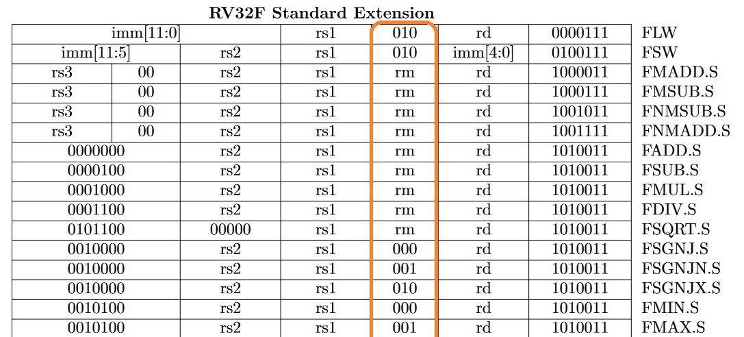
The first one is by specifying the rounding mode in an instructions. Many F/D instructions have a dedicated 3-bit field for that as shown in the following excerpt from the RISC-V ISA manual [21]:

The second option is to specify “dynamic” the instruction, which then uses the rounding mode as specified in the register FPCSR.

So, why have two ways when one suffices? As described in Design of the RISC-V Instruction Set Architecture [7], the design of the rounding mode things follow the design of most programming languages. For instance, in C++ you can set a dynamic rounding mode for following arithmetic floating point operations with std::fesetround. So pretty much the way FPCSR works. But additionally, you have non-dynamic parts. For example, casting a float value to an integer always uses roundTowardZero. So, in that case, having the rounding mode statically encoded in the instruction is beneficial.

But how often does which case arise? Again, I couldn’t find any literature, so I consulted my profiling VP. Using the VP, I tracked the rounding modes under which each instruction was executed. For the conversion instructions (float to int, int to float, etc.), the following distribution emerged:

• roundTiesToEven: 0.843
• roundTowardZero: 0.045
• roundTowardNegative: 0.056
• roundTowardPositive: 0.056
• roundTiesToAway: 4.92e-05

As you can see, roundTiesToEven is the most frequent rounding mode, while roundTiesToAway is rarely seen.

Now to arithmetic instructions (addition, multiplication, etc.):

• roundTiesToEven: 1.0
• roundTowardZero: 0.0
• roundTowardNegative: 0.0
• roundTowardPositive: 0.0
• roundTiesToAway: 0.0

Yes, you see it correctly. Out of 7,290,823,332,047 arithmetic FP instructions, not a single one used a non-default rounding mode! So, why is that? Or the better question is: Why would you use a non-default rounding mode? roundTiesToEven already gives you the smallest error, so there’s not much reason to change it.

One of the very few applications of non-default rounding modes is interval arithmetic. Using interval arithmetic, you try to determine an upper and a lower bound for your result. For example, when adding two numbers, the lower bound is given by roundTowardNegative, while the upper bound is given by roundTowardPositive. The correct result is somewhere in between. An implementation of interval arithmetic in C++ is the boost interval library [71]. Besides interval arithmetic, I couldn’t find any compelling reasons for non-default rounding in arithmetic instructions.

Ultimately, just telling from my data, having a statically encoded rounding mode in arithmetic FP instructions doesn’t make sense. If I’m missing an important aspect, please contact me!

7 Conclusion & Outlook

In this work, I showed how a modified RISC-V VP can be used to analyze the characteristics of the RISC-V FP extensions F and D. In total, the VP executed more than 16 trillion FP instructions of 78 applications, precisely tracking the distribution of FP of instructions, FP mantissa, FP exponent, and frequency of underflows.

Overall, I think the F/D extension is well-thought-out, but if I had the change to redesign it from scratch, I’d reconsider the following things:

• The FCLASS instruction seemed to be heavily underutilized. Maybe the “Zfa” extension is a more appropriate place for it.
• Non-default rounding modes for arithmetic FP instructions are extremely rare. Maybe the static rounding mode encoding in the instruction can be removed.

Besides the RISC-V-specific things, I learned the following about FP in practice:

• Most FP data is centered around a magnitude of 1
• Underflows are rare
• Loads and stores and seem to be the most common FP operations
• Having IEEE 754 is nice, but 2 revisions and lax definitions have lead to a significant fragmenation among ISAs
• Most ISAs don’t really fully adhere to IEEE 754 because it mandates too many instructions

One major ISA characteristic not analyzed in this work is the number of optimal registers. Here, the VP could be modified to track the register pressure of FP registers during the execution. But this post is already long enough, so maybe I will address it in future work.

If you found any bugs/typos or have some remarks, feel free to write me a mail. I also welcome any kind of discussion 🙂.

8 References

1. [1]L. Jünger, J. H. Weinstock, and R. Leupers, “SIM-V: Fast, Parallel RISC-V Simulation for Rapid Software Verification,” DVCON Europe 2022, 2022.
2. [2]“RISC-V ISA Dev Google Group.” [Online]. Available at: https://groups.google.com/a/groups.riscv.org/g/isa-dev
3. [3]“RISC-V ISA Manual Github Repository.” [Online]. Available at: https://github.com/riscv/riscv-isa-manual
4. [4]“RISC-V Working Groups Mailing List.” [Online]. Available at: https://lists.riscv.org/g/main
5. [5]K. Asanovic, “3rd RISC-V Workshop: RISC-V Updates.” Jan-2016 [Online]. Available at: https://riscv.org/wp-content/uploads/2016/01/Tues1000-RISCV-20160105-Updates.pdf
6. [6]T. Chen and D. A. Patterson, “RISC-V Geneology,” EECS Department, University of California, Berkeley, Tech. Rep. UCB/EECS-2016-6, 2016.
7. [7]A. Waterman, “Design of the RISC-V Instruction Set Architecture,” 2016.
8. [8]A. Waterman, Y. Lee, D. A. Patterson, and K. Asanovic, “The RISC-V Instruction Set Manual, Volume I: Base User-Level ISA, Version 1,” EECS Department, UC Berkeley, Tech. Rep. UCB/EECS-2011-62, vol. 116, 2011.
9. [9]“IEEE Standard for Floating-Point Arithmetic,” IEEE Std 754-2008. IEEE, 2008.
10. [10]“IEEE Standard for Floating-Point Arithmetic,” IEEE Std 754-2019 (Revision of IEEE 754-2008). IEEE, 2019.
11. [11]A. Waterman, Y. Lee, D. A. Patterson, and K. Asanovic, “The RISC-V Instruction Set Manual, Volume I: User-Level ISA, Version 2.2,” 2017.
12. [12]“IEEE Standard for Binary Floating-Point Arithmetic,” ANSI/IEEE Std 754-1985. IEEE, 1985.
13. [13]Intel, “80960KB Programmer’s Reference Manual.” .
14. [14]“LoongArch Reference Manual Volume 1: Basic Architecture.” .
15. [15]Intel, “Intel® IA-64 Architecture Software Developer’s Manual Volume 3: Instruction Set Reference.” 2000.
16. [16]MIPS, “MIPS® Architecture For Programmers Volume II-A: The MIPS64® Instruction Set Reference Manual Revision 6.05.” 2016.
17. [17]Intel, “Intel® 64 and IA-32 Architectures Software Developer’s Manual Volume 1: Basic Architecture.” 2016.
18. [18]IBM, “PowerPC User Instruction Set Architecture Book I Version 2.01.” 2003.
19. [19]OPENRISC.IO, “OpenRISC 1000 Architecture Manual - Architecture Version 1.3.” 2019 [Online]. Available at: https://raw.githubusercontent.com/openrisc/doc/master/openrisc-arch-1.3-rev1.pdf
20. [20]J. R. Hauser, “HardFloat Recoding.” [Online]. Available at: www.jhauser.us/arithmetic/HardFloat-1/doc/HardFloat-Verilog.html
21. [21]A. Waterman, Y. Lee, D. A. Patterson, and K. Asanovi, “The RISC-V Instruction Set Manual, Volume I: User-Level ISA, Version 2.1,” California Univ Berkeley Dept of Electrical Engineering and Computer Sciences, 2016.
22. [22]A. Waterman, “NaN Boxing Github Issue.” [Online]. Available at: https://github.com/riscv/riscv-isa-manual/issues/30
23. [23]A. Bradbury, “NaN Boxing RFC.” [Online]. Available at: https://gist.github.com/asb/a3a54c57281447fc7eac1eec3a0763fa
24. [24]A. Bradbury, “NaN Boxing ISA-Dev Group.” Mar-2017 [Online]. Available at: https://groups.google.com/a/groups.riscv.org/g/isa-dev/c/_r7hBlzsEd8/m/z1rjr2BaAwAJ
25. [25]“linpack.” [Online]. Available at: https://www.netlib.org/linpack/
26. [26]“NAS Parallel Benchmarks.” [Online]. Available at: https://www.nas.nasa.gov/software/npb.html
27. [27]“OpenNN Examples.” [Online]. Available at: https://github.com/Artelnics/opennn/tree/master/examples
28. [28]“glmark2.” [Online]. Available at: https://github.com/glmark2/glmark2
29. [29]“FinanceBench.” [Online]. Available at: https://github.com/cavazos-lab/FinanceBench
30. [30]“smallpt.” [Online]. Available at: https://github.com/matt77hias/smallpt
31. [31]“SciMark 2.0.” [Online]. Available at: https://math.nist.gov/scimark2/
32. [32]“Octane 2.0.” [Online]. Available at: https://github.com/chromium/octane
33. [33]“NumPy benchmarks.” [Online]. Available at: https://github.com/numpy/numpy/tree/main/benchmarks
34. [34]“SPEC CPU 2017.” [Online]. Available at: https://spec.org/cpu2017/
35. [35]J. Walker, “fbench.” [Online]. Available at: https://www.fourmilab.ch/fbench/fbench.html
36. [36]J. Walker, “ffbench.” [Online]. Available at: https://www.fourmilab.ch/fbench/ffbench.html
37. [37]“whetstone.” [Online]. Available at: https://netlib.org/benchmark/whetstone.c
38. [38]“STREAM benchmark.” [Online]. Available at: https://www.cs.virginia.edu/stream/
39. [39]“c-ray.” [Online]. Available at: https://github.com/jtsiomb/c-ray
40. [40]S. Fujita, “aobench.” [Online]. Available at: https://github.com/syoyo/aobench
41. [41]“Himeno Benchmark.” [Online]. Available at: https://github.com/kowsalyaChidambaram/Himeno-Benchmark
42. [42]“CoreMark®-PRO.” [Online]. Available at: https://github.com/eembc/coremark-pro
43. [43]M. R. Guthaus, J. S. Ringenberg, D. Ernst, T. M. Austin, T. Mudge, and R. B. Brown, “MiBench: A free, commercially representative embedded benchmark suite,” in Proceedings of the Fourth Annual IEEE International Workshop on Workload Characterization. WWC-4 (Cat. No.01EX538), 2001, pp. 3–14, doi: 10.1109/WWC.2001.990739.
44. [44]L. Jünger, J. H. Weinstock, and R. Leupers, “SIM-V: Fast, Parallel RISC-V Simulation for Rapid Software Verification,” DVCON Europe 2022.
45. [45]“gcov.” [Online]. Available at: https://gcc.gnu.org/onlinedocs/gcc/Gcov.html
46. [46]D. Patterson and A. Waterman, The RISC-V Reader: An Open Architecture Atlas, 1st ed. Strawberry Canyon, 2017.
47. [47]A. Akshintala, B. Jain, C.-C. Tsai, M. Ferdman, and D. E. Porter, “X86-64 Instruction Usage among C/C++ Applications,” in Proceedings of the 12th ACM International Conference on Systems and Storage, New York, NY, USA, 2019, pp. 68–79, doi: 10.1145/3319647.3325833 [Online]. Available at: https://doi.org/10.1145/3319647.3325833
48. [48]A. H. Ibrahim, M. B. Abdelhalim, H. Hussein, and A. Fahmy, “Analysis of x86 instruction set usage for Windows 7 applications,” in 2010 2nd International Conference on Computer Technology and Development, 2010, pp. 511–516, doi: 10.1109/ICCTD.2010.5645851.
49. [49]N. Bosbach, L. Jünger, R. Pelke, N. Zurstraßen, and R. Leupers, “Entropy-Based Analysis of Benchmarks for Instruction Set Simulators,” in RAPIDO2023: Proceedings of the DroneSE and RAPIDO: System Engineering for constrained embedded systems, New York, NY, USA, 2023, pp. 54–59, doi: 10.1145/3579170.3579267.
50. [50]“Analysis of X86 Instruction Set Usage for DOS/Windows Applications and Its Implication on Superscalar Design,” in Proceedings of the International Conference on Computer Design, USA, 1998, p. 566.
51. [51]D. G. Hough, “The IEEE Standard 754: One for the History Books,” Computer, vol. 52, no. 12, pp. 109–112, 2019, doi: 10.1109/MC.2019.2926614.
52. [52]“musl.” [Online]. Available at: https://musl.libc.org/
53. [53]“Newlib.” [Online]. Available at: https://sourceware.org/newlib/
54. [54]W. M. Kahan and C. Severance, “An Interview with the Old Man of Floating-Point.” [Online]. Available at: https://people.eecs.berkeley.edu/ wkahan/ieee754status/754story.html
55. [55]P. H. Sterbenz, “Floating-point computation,” 1973.
56. [56]E. M. Schwarz, M. Schmookler, and S. D. Trong, “FPU implementations with denormalized numbers,” IEEE Transactions on Computers, vol. 54, no. 7, pp. 825–836, 2005, doi: 10.1109/TC.2005.118.
57. [57]I. Dooley and L. Kale, “Quantifying the interference caused by subnormal floating-point values,” Jan. 2006.
58. [58]J. Bjørndalen and O. Anshus, “Trusting Floating Point Benchmarks - Are Your Benchmarks Really Data Independent?,” 2006, pp. 178–188, doi: 10.1007/978-3-540-75755-9_23.
59. [59]M. Wittmann, T. Zeiser, G. Hager, and G. Wellein, “Short Note on Costs of Floating Point Operations on current x86-64 Architectures: Denormals, Overflow, Underflow, and Division by Zero,” Jun. 2015.
60. [60]S. Thakkur and T. Huff, “Internet Streaming SIMD Extensions,” Computer, vol. 32, no. 12, pp. 26–34, 1999, doi: 10.1109/2.809248.
61. [61]W. M. Kahan, “Lecture Notes on the Status of IEEE Standard 754 for Binary Floating-Point Arithmetic.” [Online]. Available at: https://people.eecs.berkeley.edu/ wkahan/ieee754status/IEEE754.PDF
62. [62]J. R. Hauser, “Berkley Hardfloat Github Repository.” [Online]. Available at: https://github.com/ucb-bar/berkeley-hardfloat
63. [63]J. Gustafson and I. Yonemoto, “Beating Floating Point at its Own Game: Posit Arithmetic,” Supercomputing Frontiers and Innovations, vol. 4, pp. 71–86, Jun. 2017, doi: 10.14529/jsfi170206.
64. [64]Loyc, “Better floating point: posits in plain language.” [Online]. Available at: http://loyc.net/2019/unum-posits.html
65. [65]Wikipedia, “Wikipedia - Unum (Number Format).” [Online]. Available at: https://en.wikipedia.org/wiki/Unum_(number_format)
66. [66]J. Gustafson, “Posit arithmetic,” Mathematica Notebook describing the posit number system, 2017.
67. [67]A. Guntoro et al., “Next Generation Arithmetic for Edge Computing,” in 2020 Design, Automation and Test in Europe Conference and Exhibition (DATE), 2020, pp. 1357–1365, doi: 10.23919/DATE48585.2020.9116196.
68. [68]D. Mallasén, R. Murillo, A. A. Del Barrio, G. Botella, L. Piñuel, and M. Prieto-Matias, “PERCIVAL: Open-Source Posit RISC-V Core With Quire Capability,” IEEE Transactions on Emerging Topics in Computing, vol. 10, no. 3, pp. 1241–1252, 2022, doi: 10.1109/TETC.2022.3187199.
69. [69]J.-M. Muller et al., Handbook of Floating-Point Arithmetic. 2010.
70. [70]R. W. Hamming, “On the distribution of numbers,” The Bell System Technical Journal, vol. 49, no. 8, pp. 1609–1625, 1970, doi: 10.1002/j.1538-7305.1970.tb04281.x.
71. [71]Boost, “Boost interval.” [Online]. Available at: https://github.com/boostorg/interval